The Role of the Normal Distribution in Diffusion-Based Generative Models

I don’t fully know why, but the first time I read about the principles behind diffusion models, I really wanted to dig into them. Not the “here’s the API” level, the “why is it built this way” level.

This is the blog that came out of that.

Fair warning: this one gets fairly maths-heavy, because I like going all the way down to the scratch of how things work and why they are the way they are. I’ll explain the fundamentals as we need them, so you shouldn’t need to bring much with you.

Here’s the flow:

1. What diffusion models are at their core
2. What a distribution is, and what the Normal distribution is
3. Why Gaussian noise and not some other distribution
4. Dissecting each condition Gaussians satisfy (maths heavy)
5. Deriving the DDPM forward process closed form (maths heavy)

---

What are diffusion models at their core?

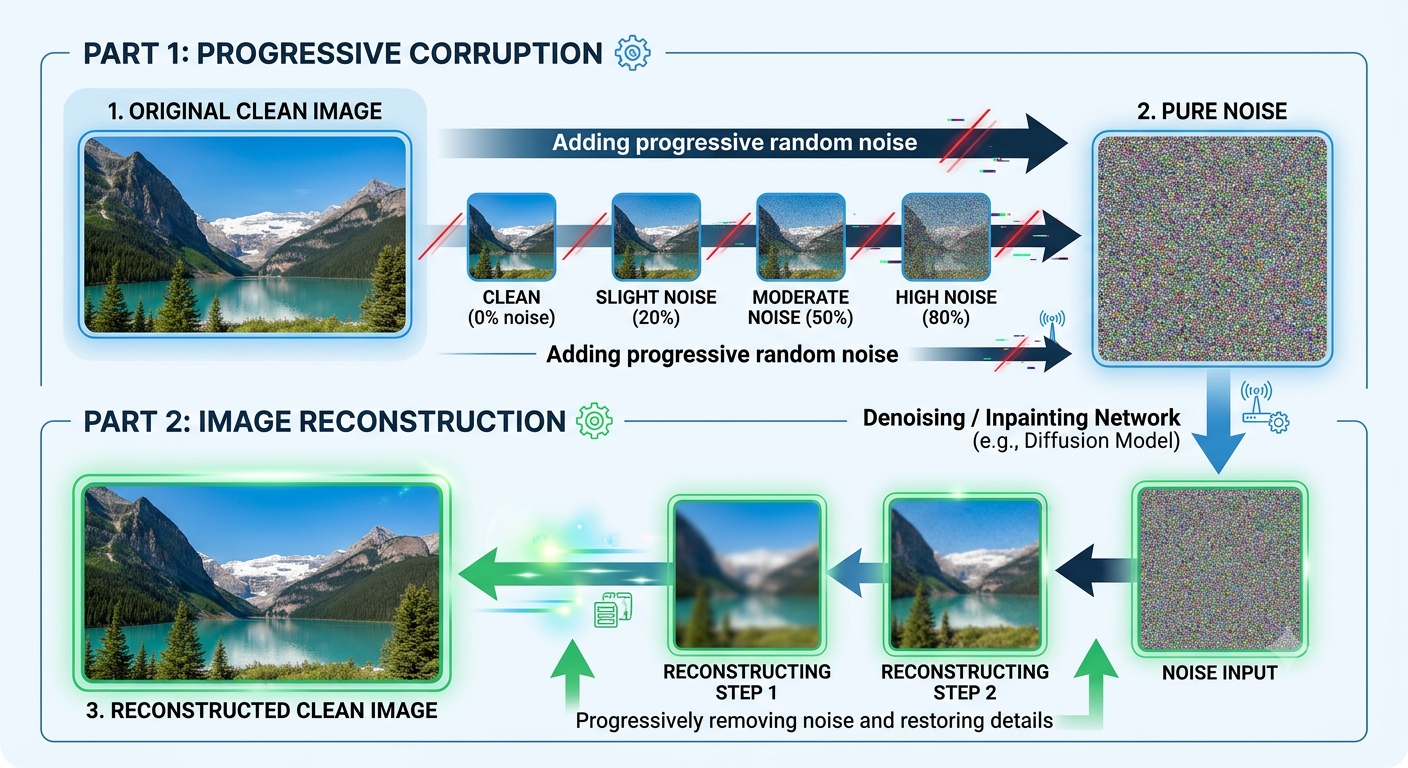
At their core, diffusion models are machines that add noise to real data, think noisy or dirty pixels in an image and then train to undo exactly that.

That’s it. You corrupt a clean image step by step, and you train a network to walk that corruption backwards until a clear image falls out.

But this blog isn’t really about diffusion model principles. It’s about a narrower and (to me) more interesting question:

What kind of noise do we add, and why?

Let me release the suspense early: we add Gaussian noise: noise that follows the Gaussian, or Normal, probability distribution.

The rest of this post is about why that choice is not arbitrary.

---

What actually is a Normal (Gaussian) distribution?

You’ve probably heard at some point that most things in the world follow a normal distribution, or some kind of bell curve.

Before the mathematics, let’s get clear on what a distribution even is.

First: what’s a distribution?

Suppose there are 1000 people in your university and you want to measure something about them like their weight, height, whatever. Let’s take height.

You measure every person, then you spread the results out:

• 15 people are 150cm
• 20 people are 155cm
• …and so on.

That’s a distribution. The table shows how height is distributed across your university. More simply: a distribution is the shape of your data.

Now: the normal distribution

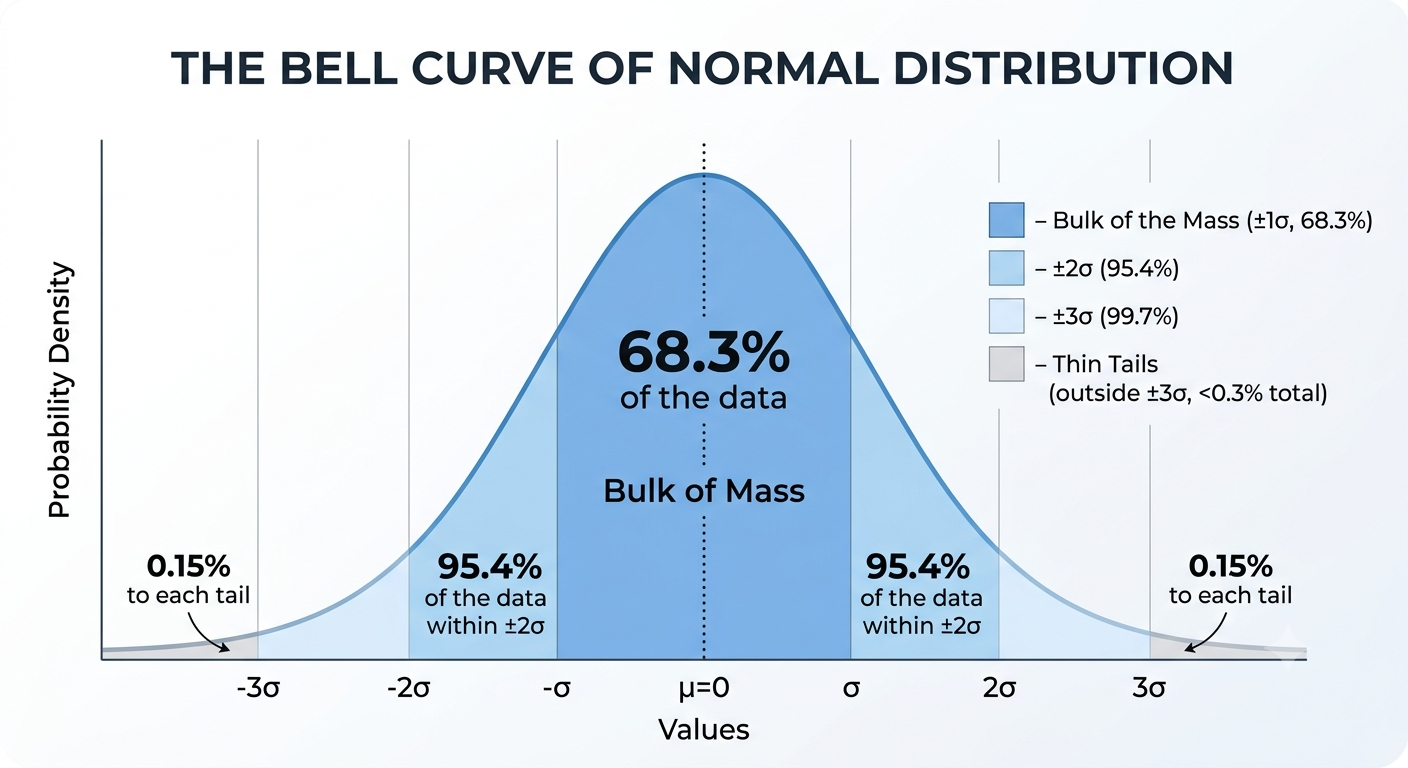
The normal distribution is the most common shape in nature, and it’s the one with the famous bell curve.

Technically: a bell-shaped distribution where most values sit near the average, and extreme values become increasingly rare.

By analogy in a class, most students are around average, a few are extremely intelligent or meritorious (like you <3), and a few are doing extremely badly (maybe they just have different interests).

That’s a normal distribution. And the key thing it says is that outliers on either side, the good side or the bad side are extremely rare.

The mathematics

The probability density function (PDF) of the normal distribution is:

$$p(x) = \frac{1}{\sqrt{2\pi\sigma^{2}}}\, \exp\!\left(-\frac{(x-\mu)^{2}}{2\sigma^{2}}\right)$$

Quick aside on what a PDF is: how much probability is packed into each tiny region. The more density in a region, the more likely a sample lands there.

Here:

• $\mu$ is the mean of the distribution — where the peak sits
• $\sigma$ is the standard deviation — how spread out it is

And we write ”$X$ is normally distributed with mean $\mu$ and variance $\sigma^2$” as:

$$X \sim \mathcal{N}(\mu, \sigma^{2})$$

---

Why Gaussian and not Uniform, or Laplace?

I’m going to answer this a bit sideways, with a proxy question that I think clears it up better:

What problem does the Gaussian distribution actually solve for us?

For diffusion models, we need a corruption process with a specific set of properties. It must:

1. Destroy structure in the data gradually and predictably step by step
2. Have a closed form for “how noisy is the data after $t$ steps” so we don’t need to simulate all $t$ steps to get to step $t$
3. Be reversible by a neural network that predicts something simple
4. Combine nicely under addition
5. Have a tractable, differentiable measure of distance between two noise distributions, so we can write a loss function
6. Eventually converge to something we can sample from analytically, with zero knowledge of the original data

The Gaussian satisfies all six. Almost nothing else does.

Point 1 is straightforward, the corruption should be predictable rather than wild, so let’s take the rest one at a time.

---

What do we mean by “the Gaussian has a closed form”?

During training, we need to show the network images at every stage of destruction. Say we want $t = 500$ out of 1000.

Without a mathematical shortcut, we’d have to start from the clean image $x_0$ and grind forward:

$$x_0 \xrightarrow{\ t_1\ } x_1 \xrightarrow{\ t_2\ } x_2 \longrightarrow \cdots \longrightarrow x_{500}$$

Five hundred sequential operations to produce one training sample. That’s brutal.

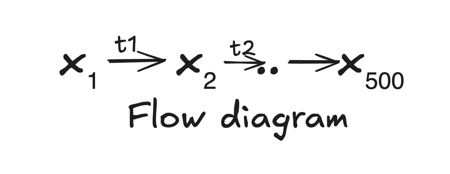
Because the Gaussian is closed under the operations we care about, we instead get a direct algebraic formula: plug in $t$, get $x_t$, compute the noisy image in a single operation.

We’ll derive that exact formula at the end of this post.

---

What do we mean by “it can be reversed by a neural network”?

A neural network in a diffusion model takes a noisy image and tries to get back to the clear one.

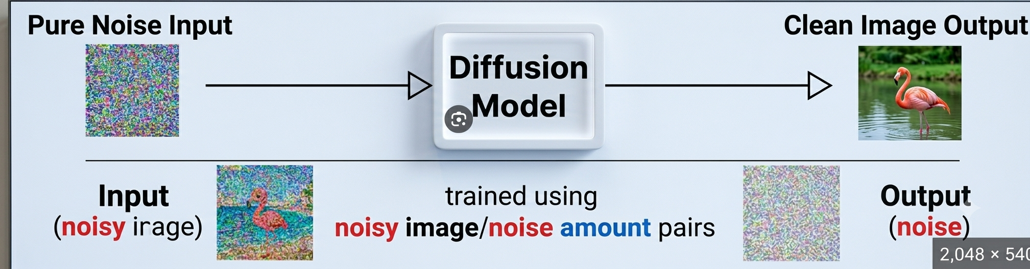
Now suppose we destroyed our image with some complex, non-Gaussian noise. Working out how to mathematically reverse that destruction is incredibly difficult.

With Gaussians, there’s a theorem that saves us:

Feller’s theorem: if a forward diffusion process takes small enough Gaussian steps, the reverse process is guaranteed to be approximately Gaussian too.

This is a big deal. Because the reverse step is Gaussian, the network only needs to predict the parameters of that Gaussian, its mean and variance. Not an arbitrary shape. Two numbers per dimension.

---

What do we mean by “it combines nicely under addition”?

Formally: closure under addition. This is the primary reason we choose Gaussian noise.

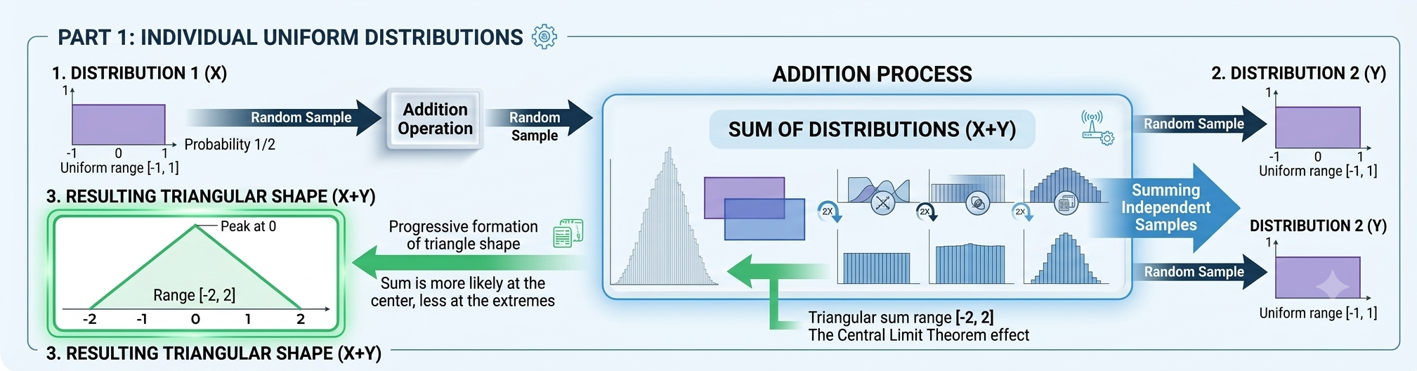
Let’s first see the problem with other distributions. Take a uniform distribution and add two of them and you get a triangular distribution. Add three and you get something else again. The shape keeps changing, and tracing your way back through it gets messy fast.

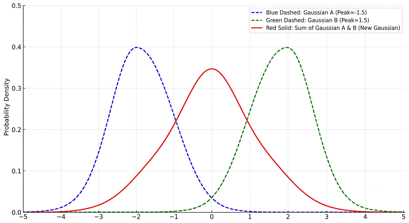
The Gaussian doesn’t do this. If we have two independent Gaussians:

$$X \sim \mathcal{N}(\mu_1, \sigma_1^{2}), \qquad Y \sim \mathcal{N}(\mu_2, \sigma_2^{2})$$

then their sum is simply another Gaussian:

$$X + Y \sim \mathcal{N}\!\left(\mu_1 + \mu_2,\ \sigma_1^{2} + \sigma_2^{2}\right)$$

(We’ll derive this properly further down, stay tuned.)

The main point: adding two independent Gaussian variables always gives a Gaussian variable, whose mean is the sum of the means and whose variance is the sum of the variances. The shape is stable. A thousand noise steps later, you’re still dealing with a Gaussian.

But wait, isn’t the image itself non-Gaussian?

There should be a doubt in your mind right now:

I get that the sum of two Gaussian noises is Gaussian. But our initial image isn’t a Gaussian, images are structured, deterministic grids of fixed pixel values. So what happens when we add noise to that?

Good question. Let’s shrink it down.

Imagine a single pixel on screen, some specific shade of grey. Give it a value of $0.8$, you probably already know every pixel is just a number.

That pixel is not random. It’s not a probability. It’s just 0.8.

Now we add Gaussian noise to it.

What happens has a name: an affine transformation.

When you take a fixed, non-random thing (a pixel with value 0.8) and add Gaussian noise to it, the fixed value doesn’t destroy the noise. It simply becomes the new centre of the noise.

An affine transformation means shifting (recentring) and scaling (stretching or shrinking). If $X$ is Gaussian and

$$Y = aX + b$$

then $Y$ is still Gaussian, $b$ shifts where it’s centred, $a$ changes how spread out it is. Precisely:

$$X \sim \mathcal{N}(\mu, \sigma^{2}) \implies Y = aX + b \sim \mathcal{N}\!\left(a\mu + b,\ a^{2}\sigma^{2}\right)$$

So: non-random value + Gaussian noise → Gaussian distribution. The determinism of the image is not a problem. It just relocates the bell curve.

---

What do we mean by “a tractable, differentiable measure of distance”?

We need to compare two things during training:

• The target: the true distribution of the reverse step
• The prediction: the network’s guessed distribution for that reverse step (also a Gaussian)

The distance between them is measured with KL divergence.

A note on KL divergence: it isn’t a true physical distance, because it isn’t symmetric, $D_{\mathrm{KL}}(p \,\|\, q) \neq D_{\mathrm{KL}}(q \,\|\, p)$. But it serves the same purpose here: measuring how different two distributions are.

(We’ll go deeper into KL divergence in another blog, stay tuned for that one.)

For two univariate Gaussians it has a clean closed form:

$$D_{\mathrm{KL}}\!\left(\mathcal{N}(\mu_1,\sigma_1^{2}) \,\big\|\, \mathcal{N}(\mu_2,\sigma_2^{2})\right) = \log\frac{\sigma_2}{\sigma_1} + \frac{\sigma_1^{2} + (\mu_1 - \mu_2)^{2}}{2\sigma_2^{2}} - \frac{1}{2}$$

Tractable here means: computable without needing infinite compute. Because both distributions are Gaussian, the maths stays simple, no integrals to approximate, no sampling to estimate the loss.

And because the KL divergence is purely algebraic for Gaussians, it’s differentiable, which means it can be backpropagated through. That’s the whole ballgame for training.

---

What do we mean by “it converges to something we can sample from”?

“Eventually” refers to the final step of our noise schedule say $T = 1000$.

At that point the mathematical system has converged onto a pure standard Gaussian, where the mean is exactly 0 and the variance is exactly 1:

$$x_T \sim \mathcal{N}(\mathbf{0}, \mathbf{I})$$

This is what makes generation possible at all. At sampling time we have no original data, we just draw pure random noise from $\mathcal{N}(\mathbf{0}, \mathbf{I})$, which anyone can do in one line of code, and let the network walk it backwards into an image.

---

Let’s get maths-heavy now

Only the Gaussian is closed under convolution

Convolution, in the context of probability, is simply the mathematical operation used to find the probability distribution of the sum of two independent random variables.

Suppose $X$ and $Y$ are two independent sources of randomness, and

$$u = X + Y$$

Then the convolution is:

$$p_{X+Y}(u) = \int_{-\infty}^{\infty} p_X(x)\, p_Y(u - x)\, dx$$

Now assume $e^{-(\text{something quadratic})}$ is the density of both $X$ and $Y$. That is:

$$p_X(x) \propto e^{-ax^{2}}, \qquad p_Y(y) \propto e^{-by^{2}}$$

Multiplying them inside the integral:

$$e^{-ax^{2} - b(u-x)^{2}}$$

and expanding that exponent:

$$-ax^{2} - b(u-x)^{2} = -(a+b)x^{2} + 2bux - bu^{2}$$

which is still a quadratic. That’s the whole trick. A quadratic in the exponent goes in, a quadratic in the exponent comes out, so a Gaussian goes in and a Gaussian comes out. The family is closed.

---

Deriving the sum of two Gaussians via the full convolution integral

Let’s actually do it properly.

Setup. Let

$$X \sim \mathcal{N}(\mu_1, \sigma_1^{2}), \qquad Y \sim \mathcal{N}(\mu_2, \sigma_2^{2}), \qquad Z = X + Y$$

with densities

$$p_X(x) = \frac{1}{\sqrt{2\pi\sigma_1^{2}}}\, e^{-\frac{(x-\mu_1)^{2}}{2\sigma_1^{2}}}, \qquad p_Y(y) = \frac{1}{\sqrt{2\pi\sigma_2^{2}}}\, e^{-\frac{(y-\mu_2)^{2}}{2\sigma_2^{2}}}$$

Step 1 is write the convolution.

$$p_Z(z) = \int_{-\infty}^{\infty} p_X(x)\, p_Y(z-x)\, dx$$ $$p_Z(z) = \int_{-\infty}^{\infty} \left[\frac{1}{\sqrt{2\pi\sigma_1^{2}}} e^{-\frac{(x-\mu_1)^{2}}{2\sigma_1^{2}}}\right] \left[\frac{1}{\sqrt{2\pi\sigma_2^{2}}} e^{-\frac{(z-x-\mu_2)^{2}}{2\sigma_2^{2}}}\right] dx$$

Pulling the constants out:

$$p_Z(z) = \frac{1}{2\pi\sigma_1\sigma_2} \int_{-\infty}^{\infty} e^{-\frac{(x-\mu_1)^{2}}{2\sigma_1^{2}} - \frac{(z-x-\mu_2)^{2}}{2\sigma_2^{2}}}\, dx$$

Step 2 is substitute to clean it up. Let

$$w = x - \mu_1 \quad (dw = dx), \qquad v = z - (\mu_1 + \mu_2)$$

Then the exponent becomes:

$$\text{exponent} = -\frac{1}{2}\left[\frac{w^{2}}{\sigma_1^{2}} + \frac{v^{2} - 2vw + w^{2}}{\sigma_2^{2}}\right]$$

Step 3 is group by powers of $w$.

$$= -\frac{1}{2}\left[w^{2}\!\left(\frac{1}{\sigma_1^{2}} + \frac{1}{\sigma_2^{2}}\right) - w\!\left(\frac{2v}{\sigma_2^{2}}\right) + \frac{v^{2}}{\sigma_2^{2}}\right]$$

Now define $\sigma^{2} = \sigma_1^{2} + \sigma_2^{2}$, which lets us write $\frac{1}{\sigma_1^2} + \frac{1}{\sigma_2^2} = \frac{\sigma^2}{\sigma_1^2\sigma_2^2}$:

$$= -\frac{1}{2}\left[w^{2}\!\left(\frac{\sigma^{2}}{\sigma_1^{2}\sigma_2^{2}}\right) - 2w\!\left(\frac{v}{\sigma_2^{2}}\right) + \frac{v^{2}}{\sigma_2^{2}}\right]$$

Step 4 is complete the square in $w$.

$$= -\frac{1}{2}\left[\frac{\sigma^{2}}{\sigma_1^{2}\sigma_2^{2}}\left(w - \frac{v\sigma_1^{2}}{\sigma^{2}}\right)^{2} + \frac{v^{2}}{\sigma^{2}}\right]$$

The second term has no $w$ in it, so it escapes the integral:

$$p_Z(z) = \frac{1}{2\pi\sigma_1\sigma_2}\, e^{-\frac{v^{2}}{2\sigma^{2}}} \int_{-\infty}^{\infty} e^{-\frac{\sigma^{2}}{2\sigma_1^{2}\sigma_2^{2}}\left(w - \frac{v\sigma_1^{2}}{\sigma^{2}}\right)^{2}} dw$$

Step 5 is evaluate using the Gaussian integral. Recall:

$$\int_{-\infty}^{\infty} e^{-Au^{2}}\, du = \sqrt{\frac{\pi}{A}}, \qquad \text{here } A = \frac{\sigma^{2}}{2\sigma_1^{2}\sigma_2^{2}}$$

So the integral evaluates to:

$$\sqrt{\frac{2\pi\sigma_1^{2}\sigma_2^{2}}{\sigma^{2}}}$$

Step 6 is put it together and watch it collapse.

$$p_Z(z) = \frac{1}{2\pi\sigma_1\sigma_2}\left[\sqrt{\frac{2\pi\sigma_1^{2}\sigma_2^{2}}{\sigma^{2}}}\right] e^{-\frac{v^{2}}{2\sigma^{2}}} = \frac{1}{\sqrt{2\pi\sigma^{2}}}\, e^{-\frac{v^{2}}{2\sigma^{2}}}$$

Substituting back $v = z - (\mu_1 + \mu_2)$ and $\sigma^{2} = \sigma_1^{2} + \sigma_2^{2}$:

$$p_Z(z) = \frac{1}{\sqrt{2\pi(\sigma_1^{2} + \sigma_2^{2})}}\, \exp\!\left(-\frac{\big(z - (\mu_1 + \mu_2)\big)^{2}}{2(\sigma_1^{2} + \sigma_2^{2})}\right)$$

which is exactly the density of

$$\boxed{\;Z = X + Y \sim \mathcal{N}\!\left(\mu_1 + \mu_2,\ \sigma_1^{2} + \sigma_2^{2}\right)\;}$$

Means add. Variances add. And critically it’s still a Gaussian.

---

Why $-(\text{quadratic})$ and not something else?

A quick but important detour. Why does the exponent need to be negative quadratic?

A parabola of the form

$$-a(x - \mu)^{2} + c, \qquad a > 0$$

is a downward parabola. That’s what keeps the integrand from exploding.

If $a$ could be any value — suppose $a < 0$, then as $x \to \pm\infty$ the exponent $\to +\infty$, so the whole integrand $e^{-(\text{quadratic})} \to e^{+\infty}$. It blows up, the integral diverges, and it’s not a probability density at all.

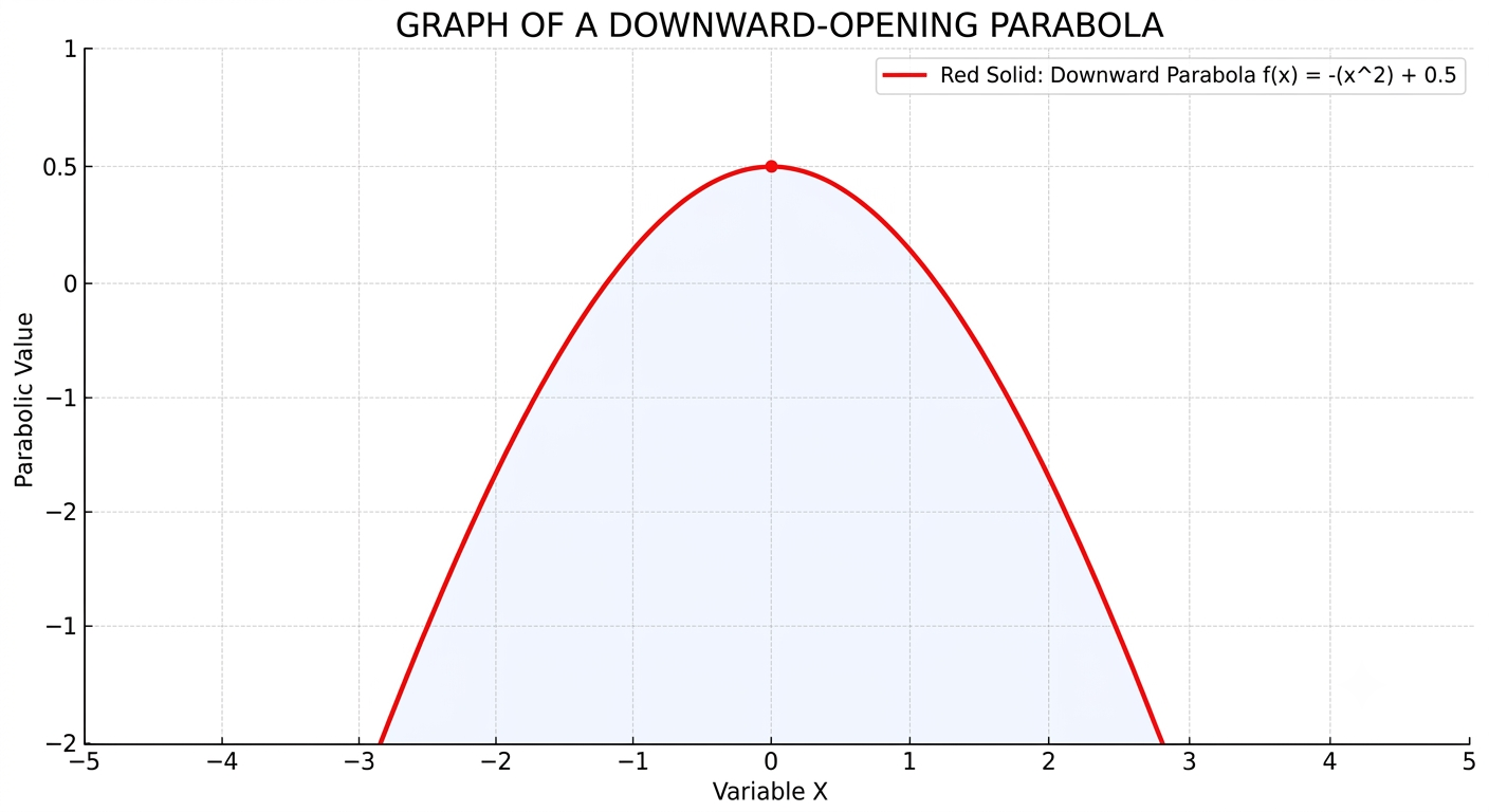
So in $-a(x-\mu)^2 + c$:

• $\mu$ is the location of the peak
• $a$ decides how fast it decays (and must satisfy $a > 0$)

---

The multivariate case

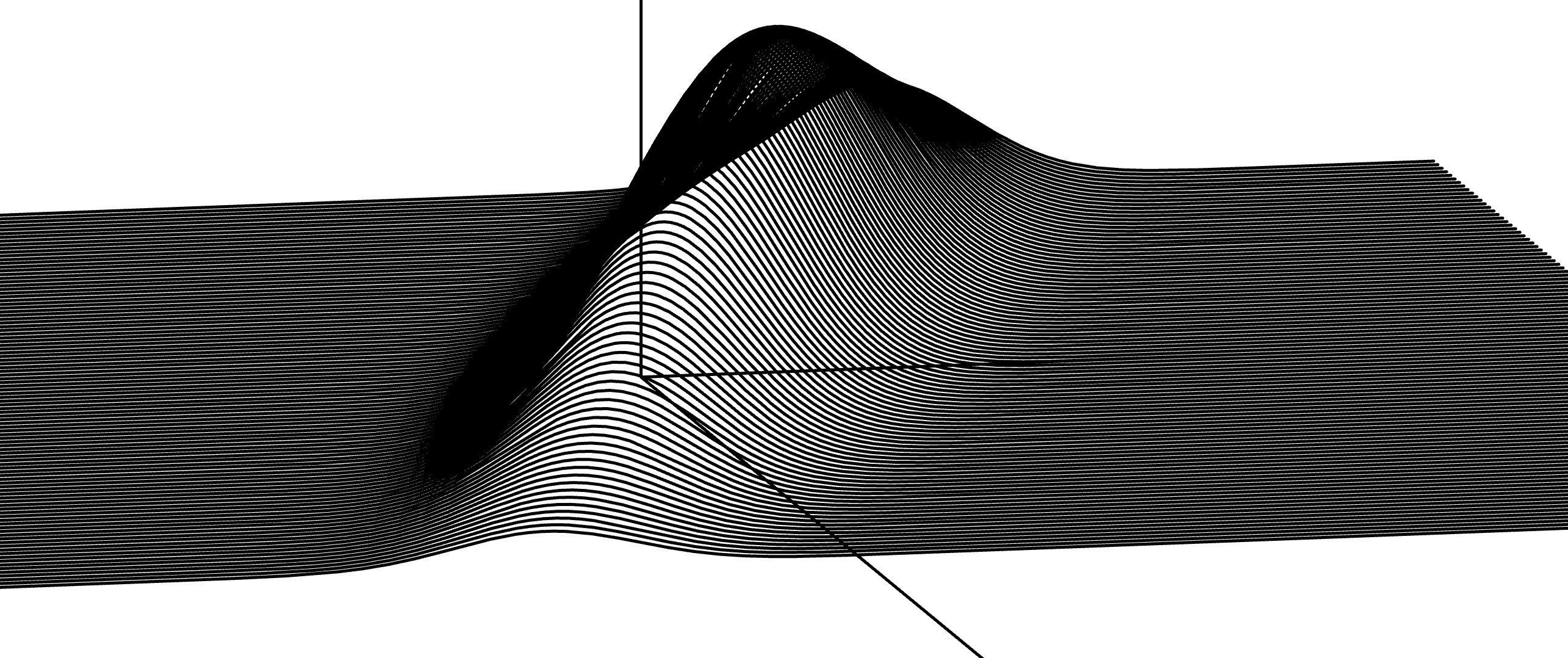
An important point: real-world noise isn’t univariate Gaussian, it’s multivariate. An image isn’t one number, it’s hundreds of thousands of them.

The multivariate Gaussian density is:

$$p(\mathbf{x}) = \frac{1}{(2\pi)^{d/2}\,|\boldsymbol{\Sigma}|^{1/2}} \exp\!\left(-\frac{1}{2}(\mathbf{x} - \boldsymbol{\mu})^{\top} \boldsymbol{\Sigma}^{-1} (\mathbf{x} - \boldsymbol{\mu})\right)$$

where:

• $\boldsymbol{\mu} \in \mathbb{R}^{d}$ : a mean vector instead of a single mean
• $\boldsymbol{\Sigma} \in \mathbb{R}^{d \times d}$ : the covariance matrix, a symmetric positive semi-definite matrix

with entries

$$\Sigma_{i,j} = \mathbb{E}\big[(x_i - \mu_i)(x_j - \mu_j)\big]$$

(If positive semi-definite matrices are new to you, they’re worth a look, they show up constantly in optimisation theory.)

---

Why do diffusion models always use $\boldsymbol{\Sigma} = \sigma^{2}\mathbf{I}$?

In practice, diffusion models don’t use a general covariance matrix. They use an isotropic one:

$$\sigma^{2}\mathbf{I} = \begin{bmatrix} \sigma^{2} & 0 & \cdots & 0 \\ 0 & \sigma^{2} & \cdots & 0 \\ \vdots & \vdots & \ddots & \vdots \\ 0 & 0 & \cdots & \sigma^{2} \end{bmatrix}$$

Isotropic is a concept borrowed from physics: something that looks the same in every direction.

What this assumes is that pixels are independent and identically distributed. Concretely:

• adding noise to the top-left pixel has zero effect on the noise added to the bottom-right pixel
• every single pixel gets hit with the exact same severity of noise, $\sigma^2$

In reality, pixels aren’t independent at all. Neighbouring pixels in a real photo are enormously correlated. So why make an assumption we know is false?

Because the alternative is computationally impossible. A full covariance matrix requires the relationship between every pixel and every other pixel, simultaneously. For a 1-megapixel image, that grid has $10^{6} \times 10^{6} = 10^{12}$ entries ie. a trillion numbers, for a single noise step. No hardware is doing that.

The isotropic assumption also collapses the matrix inverse:

$$\boldsymbol{\Sigma}^{-1} = \frac{1}{\sigma^{2}}\mathbf{I}$$

This matters more than it looks. Inverting a general $d \times d$ matrix costs roughly $O(d^3)$ operations and is numerically fragile, small errors get amplified badly. But the density formula above needs $\boldsymbol{\Sigma}^{-1}$, and it needs it constantly. With an isotropic covariance, that inversion becomes dividing by a scalar. An $O(d^3)$ problem becomes an $O(1)$ one.

---

The payoff: deriving the DDPM forward process closed form

Now let’s apply everything we’ve built.

To train a diffusion model, we start with a clean image and slowly destroy it over $T$ steps.

At any single step $t$, we take the image from the immediately previous step ($x_{t-1}$), scale its pixel values down just a tiny bit (by $\sqrt{1 - \beta_t}$), and add a tiny splash of new noise ($\beta_t$):

$$q(x_t \mid x_{t-1}) = \mathcal{N}\!\left(x_t;\ \sqrt{1 - \beta_t}\, x_{t-1},\ \beta_t \mathbf{I}\right)$$

Reparameterisation

Sampling from that distribution is the same as writing:

$$x_t = \sqrt{1 - \beta_t}\; x_{t-1} + \sqrt{\beta_t}\; \epsilon_t, \qquad \epsilon_t \sim \mathcal{N}(\mathbf{0}, \mathbf{I}) \tag{i}$$

where $\beta_t \in (0, 1)$, $x_t$ is the new image at step $t$, and $x_{t-1}$ is the old image at step $t-1$.

This is just the affine transformation from earlier, applied once per step.

Unrolling the recursion

Let $\alpha_t = 1 - \beta_t$. Then:

$$x_t = \sqrt{\alpha_t}\, x_{t-1} + \sqrt{1 - \alpha_t}\; \epsilon_t$$

And the same relation one step earlier:

$$x_{t-1} = \sqrt{\alpha_{t-1}}\, x_{t-2} + \sqrt{1 - \alpha_{t-1}}\; \epsilon_{t-1}$$

Substituting the second into the first:

$$x_t = \sqrt{\alpha_t \alpha_{t-1}}\; x_{t-2} \;+\; \underbrace{\sqrt{\alpha_t(1 - \alpha_{t-1})}\; \epsilon_{t-1} + \sqrt{1 - \alpha_t}\; \epsilon_t}_{\text{sum of two independent Gaussians}}$$

And here’s where all that convolution work pays off. Those two noise terms are independent Gaussians, both with mean 0. By the result we derived, their sum is a single Gaussian whose variances add:

$$\mu_1 + \mu_2 = 0 + 0 = 0$$ $$\sigma_1^2 + \sigma_2^2 = \left(\sqrt{\alpha_t(1 - \alpha_{t-1})}\right)^{2} + \left(\sqrt{1 - \alpha_t}\right)^{2} = \alpha_t(1 - \alpha_{t-1}) + (1 - \alpha_t)$$

which simplifies beautifully:

$$\alpha_t - \alpha_t\alpha_{t-1} + 1 - \alpha_t = 1 - \alpha_t \alpha_{t-1}$$

So the two noise terms collapse into one:

$$\text{new Gaussian} \sim \mathcal{N}\!\left(0,\ 1 - \alpha_t \alpha_{t-1}\right)$$

Two noise terms became one. Do this again and three become one. Keep unrolling all the way down to $x_0$ and every noise term in the entire chain collapses into a single Gaussian.

The closed form

Define the cumulative product $\bar{\alpha}_t = \prod_{s=1}^{t} \alpha_s$. Then:

$$\boxed{\;x_t = \sqrt{\bar{\alpha}_t}\; x_0 + \sqrt{1 - \bar{\alpha}_t}\; \epsilon, \qquad \epsilon \sim \mathcal{N}(\mathbf{0}, \mathbf{I})\;}$$

This is the whole point. Want the image at $t = 500$? You don’t simulate 500 steps. You look up $\bar{\alpha}_{500}$, draw one sample of noise, and compute it in a single operation.

And look at what each piece does:

• $\sqrt{\bar{\alpha}_t}$ shrinks toward 0 as $t$ grows → the original image fades out
• $\sqrt{1 - \bar{\alpha}_t}$ grows toward 1 → the noise takes over

At $t = T$, $\bar{\alpha}_T \approx 0$, and we’re left with $x_T \approx \epsilon \sim \mathcal{N}(\mathbf{0}, \mathbf{I})$ , exactly the pure standard Gaussian we promised in condition 6, that we can sample from with zero knowledge of the original data.

---

Wrapping up

So, why Gaussian noise?

Not because it’s traditional, and not because it’s the noise nature happens to produce. Because it’s the only distribution that gives us all six properties at once:

Property	What the Gaussian gives us
Gradual, predictable destruction	A controllable variance schedule $\beta_t$
Closed form at step $t$	$x_t = \sqrt{\bar{\alpha}_t}x_0 + \sqrt{1-\bar{\alpha}_t}\,\epsilon$
Reversible by a network	Feller’s theorem — reverse step is also Gaussian
Combines under addition	Closed under convolution; means and variances add
Differentiable loss	KL divergence between Gaussians is algebraic
Analytically samplable limit	Converges to $\mathcal{N}(\mathbf{0}, \mathbf{I})$

Every one of those traces back to the same underlying fact: a quadratic in the exponent stays a quadratic. That single algebraic property is what makes the entire architecture tractable.

Next up, I want to go deeper into Probability Theory and Information Theory(Concepts like Entropy, KL Divergence, Cross Entropy ,etc).